
Packed-bed model#
PackedBedModel describes a bed of spherical PCM capsules with the heat transfer fluid
flowing through the voids. At each point along the bed, heat conducts across a capsule
(resolved radially) and into the fluid at its surface. It is built from the same submodels
as the finned-tube models, so it has the same outputs, conserves energy exactly and runs the same experiments.
The default parameters are the experiments of Nallusamy et al. (2007): a 47 l tank of paraffin capsules in water, charged with water at 70 °C from 32 °C.
For the geometry, the equations and the options of the packed-bed model, with sketches, see the Packed bed page of the documentation.
Tutorial 3 introduces this model.
import matplotlib.pyplot as plt
import numpy as np
import pybamm

import pytes

model = pytes.PackedBedModel()
model.print_submodel_info()
fluid: AdvectedFluid (Heat transfer fluid)
    requires:
        Heat transfer fluid heat gain per unit length [W.m-1]
        Initial uniform temperature [K]
    provides:
        Heat transfer fluid specific enthalpy [J.kg-1]
        Inlet specific enthalpy [J.kg-1]
        Outlet specific enthalpy [J.kg-1]
        Mass flow rate [kg.s-1]
        Heat transfer fluid thermal energy [J]
        Heat transfer fluid temperature [K]
        Inlet temperature [K]
        Outlet temperature [K]
        Inlet-outlet temperature difference [K]
        Heat transfer fluid velocity [m.s-1]
        Volume flow rate [m3.s-1]
        Pumped volume [m3]
    parameters:
        Bed cross-sectional area [m2]
        Bed length [m]
        Bed porosity
        Heat transfer fluid density [kg.m-3]
        Heat transfer fluid specific heat capacity [J.kg-1.K-1]
        Inlet temperature [K]
        Mass flow rate [kg.s-1]
        PCM melting temperature [K]
        Reference temperature [K]
    assumptions:
        The fluid is incompressible, with constant density.
        Axial conduction and dispersion in the fluid are neglected.
        The flow is the same in every flow path.
storage: EnthalpyStorage (Phase-change material storage)
    requires:
        Phase-change material boundary heat flux [W.m-2]
        Initial uniform temperature [K]
    provides:
        Phase-change material enthalpy [J.m-3]
        Phase-change material enthalpy rate of change [W.m-3]
        Phase-change material conduction heating rate [W.m-3]
        Phase-change material thermal energy [J]
        Liquid fraction
        Phase
        Average liquid fraction
        Phase-change material temperature [K]
        Phase-change material average temperature [K]
        Phase-change material cross-section average temperature [K]
        Phase-change material surface temperature [K]
        Phase-change material thermal conductivity [W.m-1.K-1]
    parameters:
        Bed cross-sectional area [m2]
        Bed porosity
        Capsule radius [m]
        PCM latent heat [J.kg-1]
        PCM liquid phase conductivity [W.m-1.K-1]
        PCM liquid phase density [kg.m-3]
        PCM liquid phase specific heat capacity [J.kg-1.K-1]
        PCM melting range [K]
        PCM melting temperature [K]
        PCM smoothing width [K]
        PCM solid phase conductivity [W.m-1.K-1]
        PCM solid phase density [kg.m-3]
        PCM solid phase specific heat capacity [J.kg-1.K-1]
        Reference temperature [K]
    assumptions:
        Heat flows along the primary spatial variable only.
        Heat flows by conduction only (no convection in the liquid).
        The volume change on melting is neglected.
coupling: WallCoupling (Wall coupling)
    requires:
        Phase-change material conduction heating rate [W.m-3]
        Heat transfer fluid specific enthalpy [J.kg-1]
        Heat transfer fluid temperature [K]
        Phase-change material surface temperature [K]
        Mass flow rate [kg.s-1]
    provides:
        Heat transfer fluid heat gain per unit length [W.m-1]
        Phase-change material boundary heat flux [W.m-2]
        Heat transfer coefficient [W.m-2.K-1]
        Surface Reynolds number
        Surface Prandtl number
    parameters:
        Bed cross-sectional area [m2]
        Bed porosity
        Capsule radius [m]
        Heat transfer coefficient [W.m-2.K-1]
        Heat transfer fluid conductivity [W.m-1.K-1]
        Heat transfer fluid specific heat capacity [J.kg-1.K-1]
        Heat transfer fluid viscosity [Pa.s]
    assumptions:
        (none)
device energy: DeviceEnergy (Device energy)
    requires:
        Mass flow rate [kg.s-1]
        Outlet specific enthalpy [J.kg-1]
        Inlet specific enthalpy [J.kg-1]
        Phase-change material thermal energy [J]
        Heat transfer fluid thermal energy [J]
        Phase-change material average temperature [K]
        Phase-change material cross-section average temperature [K]
    provides:
        Power [W]
        Discharged energy [J]
        Charged energy [J]
        Discharged throughput [J]
        Charged throughput [J]
        Storage thermal energy [J]
        Total thermal energy [J]
        Heat loss power [W]
        Storage average temperature [K]
        Storage cross-section average temperature [K]
        Initial uniform temperature [K]
    parameters:
        Initial temperature [K]
    assumptions:
        There are no heat losses to the surroundings.
per-area totals: PerAreaTotals (Per-area totals)
    requires:
        Power [W]
        Discharged energy [J]
        Storage thermal energy [J]
        Total thermal energy [J]
    provides:
        Power per unit area [W.m-2]
        Discharged energy per unit area [J.m-2]
        Storage thermal energy per unit area [J.m-2]
        Total thermal energy per unit area [J.m-2]
    parameters:
        Bed cross-sectional area [m2]
    assumptions:
        (none)
geometry parameters:
    Bed length [m]
    Capsule radius [m]
t_end = 160 * 60
solution = pybamm.Simulation(model).solve(
    [0, t_end], t_interp=np.linspace(0, t_end, 321)
)
E = solution["Total thermal energy [J]"].entries
discharged = solution["Discharged energy [J]"].entries
print("max conservation error [J]:", np.max(np.abs(E - E[0] + discharged)))
print("stored energy [kWh]:", E[-1] / 3.6e6)
print(
    "energy between 32 and 70 degC [kWh]:",
    pytes.energy_between(model, 273.15 + 32, 273.15 + 70) / 3.6e6,
)
print(
    "stored energy per unit area [MJ.m-2]:",
    solution["Total thermal energy per unit area [J.m-2]"].entries[-1] / 1e6,
)
max conservation error [J]: 2.60770320892334e-08
stored energy [kWh]: 2.3031771680909383
energy between 32 and 70 degC [kWh]: 2.635389843901675
stored energy per unit area [MJ.m-2]: 81.45822913734806
The measured fluid temperatures at a quarter, half, three quarters and the full height of the bed (points) against the model (lines).
Z = model.default_parameter_values["Bed length [m]"]
fig, ax = plt.subplots(figsize=(6, 4))
for position, fraction in [("0.25L", 0.25), ("0.5L", 0.5), ("0.75L", 0.75), ("1L", 1)]:
    t_data, T_data = np.loadtxt(
        f"data/Nallusamy2007_HTF_{position}.csv", delimiter=",", skiprows=1, unpack=True
    )
    t = solution["Time [s]"].entries
    T = solution["Heat transfer fluid temperature [degC]"](t=t, z=fraction * Z)
    (line,) = ax.plot(t / 60, T, label=f"{fraction:g} L")
    ax.plot(t_data, T_data, "o", color=line.get_color(), markersize=3)
ax.set_xlabel("Time [min]")
ax.set_ylabel("Fluid temperature [°C]")
ax.legend()
plt.show()
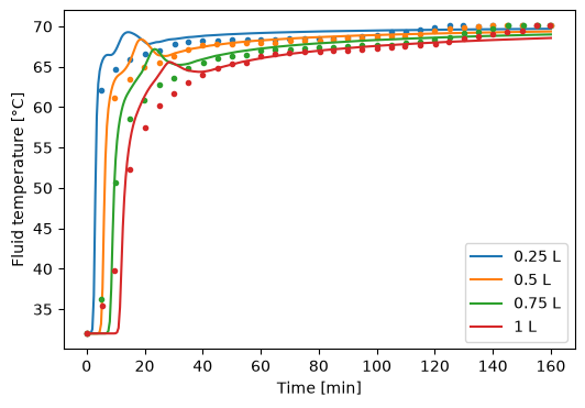
The fluid temperatures agree with the measurements to 1 K to 2 K (root mean square). Inside the capsules the agreement is looser, about 5 K at 0.8 of the capsule radius, which depends on where the thermocouples sat and on the capsule shell, which the model neglects.
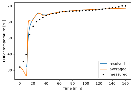
With options={"storage along flow path": "averaged"}, one capsule stands for the average along the bed and
exchanges heat with the fluid averaged along it: much faster, but it cannot capture the
thermal front moving through the bed. Every model has this option.
Note the dip of the averaged outlet below the initial 32 °C early on: the heat the capsule takes from the averaged fluid is taken uniformly along the bed, including near the outlet, where the fluid is still cold. This is a known artefact of this formulation, the published reduced model; energy is still conserved exactly.
averaged = pytes.PackedBedModel(options={"storage along flow path": "averaged"})
averaged_solution = pybamm.Simulation(averaged).solve(
    [0, t_end], t_interp=np.linspace(0, t_end, 321)
)
print(
    f"solve time: resolved {solution.solve_time}, averaged {averaged_solution.solve_time}"
)

t_data, T_data = np.loadtxt(
    "data/Nallusamy2007_HTF_1L.csv", delimiter=",", skiprows=1, unpack=True
)
fig, ax = plt.subplots(figsize=(6, 4))
for sol, label in [(solution, "resolved"), (averaged_solution, "averaged")]:
    ax.plot(
        sol["Time [min]"].entries, sol["Outlet temperature [degC]"].entries, label=label
    )
ax.plot(t_data, T_data, "ko", markersize=3, label="measured")
ax.set_xlabel("Time [min]")
ax.set_ylabel("Outlet temperature [°C]")
ax.legend()
plt.show()
solve time: resolved 1.532 s, averaged 75.950 ms