Tutorial 5: plotting

There are three ways to plot a PyTES solution:

1. PyBaMM’s QuickPlot, for a quick look at any outputs, with a slider for time;

2. the standard plots of pytes.plotting, which compare designs the same way every time;

3. your own matplotlib figures, from the values in the solution.

All three work on the same solutions. Here they are a discharge of the finned-tube battery (Tutorial 2) and a charge of the packed bed (Tutorial 3).

import matplotlib.pyplot as plt
import numpy as np
import pybamm

import pytes
from pytes import plotting

t_eval = np.linspace(0, 3600, 121)
finned = pybamm.Simulation(pytes.SharpFrontModel()).solve([0, 3600], t_interp=t_eval)
bed = pybamm.Simulation(pytes.PackedBedModel()).solve([0, 3600], t_interp=t_eval)

QuickPlot

pybamm.dynamic_plot plots any outputs of one or more solutions, by name, with a slider for time. Outputs in a nested list share an axis. Outputs that vary in space, such as the fluid temperature along the flow path, are drawn at the time of the slider.

pybamm.dynamic_plot(
    finned,
    [
        ["Inlet temperature [degC]", "Outlet temperature [degC]"],
        "Heat transfer fluid temperature [degC]",
        "Power [kW]",
        "Average liquid fraction",
    ],
    time_unit="minutes",
    spatial_unit="m",
);

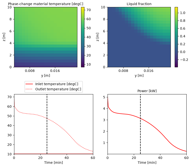
For a static figure at a chosen time, as in a report, build a pybamm.QuickPlot and call its plot method with the time, in the plot’s time unit. Outputs that vary in two dimensions are drawn as a map, here the temperature and the liquid fraction across the storage and along the tube, after 25 minutes.

quick_plot = pybamm.QuickPlot(
    finned,
    [
        "Phase-change material temperature [degC]",
        "Liquid fraction",
        ["Inlet temperature [degC]", "Outlet temperature [degC]"],
        "Power [kW]",
    ],
    time_unit="minutes",
    spatial_unit="m",
)
quick_plot.plot(25)

Standard plots

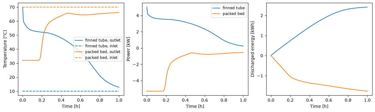
pytes.plotting (installed with pip install "pytes-thermal[plot]") has the plots used most often to compare designs. Every model has the same outputs, so they apply to any model. plot_summary gives the inlet and outlet temperatures, the power and the discharged energy; the bed is charging, so its power and discharged energy are negative.

fig, axes = plotting.plot_summary([finned, bed], labels=["finned tube", "packed bed"])
plt.show()

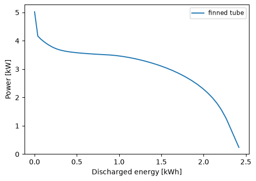
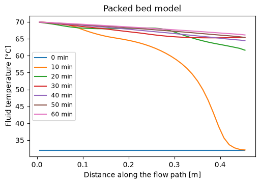
plot_power_against_energy shows how the power a battery delivers falls as it gives up its energy, the key comparison between designs. plot_fluid_profiles gives the fluid temperature along the flow path at chosen times, here the thermal front moving up the bed.

plotting.plot_power_against_energy(finned, labels=["finned tube"])
plotting.plot_fluid_profiles(bed, [0, 600, 1200, 1800, 2400, 3000, 3600])
plt.show()

Your own figures

Each output in the solution gives its values at the solution times with .entries. Calling an output gives its value at any time, and at any position for the outputs that vary in space (z along the flow path, y across the storage of a finned tube, r across a capsule). Positions outside the mesh points, output.mesh.nodes, are extrapolated, so it is best to stay within them. 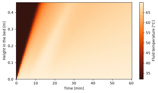With these, any matplotlib figure is a few lines. Here the fluid temperature along the bed over time is drawn as a map, with the PyTES colourmap ember (see the plot colours example for the colour cycles and colourmaps).

Z = pytes.PackedBedModel().default_parameter_values["Bed length [m]"]
fluid = bed["Heat transfer fluid temperature [degC]"]
z = fluid.mesh.nodes
T = fluid(t=t_eval, z=z)

fig, ax = plt.subplots(figsize=(6, 3.5), layout="constrained")
field = ax.pcolormesh(t_eval / 60, z, T, cmap="pytes.ember", shading="nearest")
fig.colorbar(field, label="Fluid temperature [°C]")
ax.set_xlabel("Time [min]")
ax.set_ylabel("Height in the bed [m]")
plt.show()

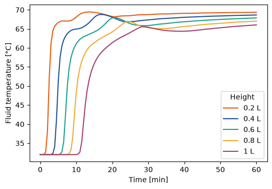
The PyTES colour cycle applies to any figure with a matplotlib style, for one figure with plt.style.context("pytes.thermal") or for every figure with plt.style.use("pytes.thermal").

with plt.style.context("pytes.thermal"):
    fig, ax = plt.subplots(figsize=(6, 4))
    for fraction in [0.2, 0.4, 0.6, 0.8, 1]:
        ax.plot(
            t_eval / 60,
            bed["Heat transfer fluid temperature [degC]"](t=t_eval, z=fraction * Z),
            label=f"{fraction:g} L",
        )
    ax.set_xlabel("Time [min]")
    ax.set_ylabel("Fluid temperature [°C]")
    ax.legend(title="Height")
    plt.show()

Next: Tutorial 6: experiments.