Tutorial 6: experiments

So far each model ran with fixed operating conditions: a constant inlet temperature and mass flow rate. An experiment operates a battery the way it is used or tested, as a sequence of steps, such as “discharge at 2 kW until the outlet falls below 40 °C, rest for an hour, then charge”.

A heat battery has two controls, the inlet temperature and the mass flow rate. There are three kinds of step:

• Inlet holds both controls;

• Rest stops the flow;

• Power holds the power, by adjusting the control you do not give.

Each step ends after its duration or when one of its termination conditions is met. run_experiment runs the steps in order and returns an ordinary pybamm.Solution.

import numpy as np
import pybamm

import pytes
from pytes import plotting
from pytes.experiments import Experiment, run_experiment
from pytes.experiments import step as s

model = pytes.SharpFrontModel()
T_cold, T_hot = 273.15 + 10, 273.15 + 75

A first experiment

Temperatures are in kelvin, mass flow rates in kg/s and times in seconds. This step is the default discharge of the earlier tutorials (see Tutorial 2), water at 10 °C and 0.02 kg/s, but it stops when the outlet falls below 40 °C, the lowest useful temperature for hot water, instead of after an hour.

discharge = s.Inlet(T_cold, 0.02, termination=s.outlet_temperature_below(273.15 + 40))
solution = run_experiment(model, Experiment([discharge]))
print(
    f"hot water for {solution['Time [min]'].entries[-1]:.0f} min, "
    f"{solution['Discharged energy [kWh]'].entries[-1]:.2f} kWh delivered"
)

hot water for 34 min, 1.90 kWh delivered

Holding the power

A Power step holds the power of the battery, positive on discharge and negative on charge. Give it one control and it adjusts the other. Here the inlet is held at 10 °C and the flow adjusts to deliver 2 kW: it rises as the battery cools. The flow needed grows without bound as the outlet approaches the inlet temperature, so the step also stops if the flow exceeds 0.1 kg/s.

constant_power = s.Power(
    2e3,
    inlet_temperature=T_cold,
    termination=[
        s.outlet_temperature_below(273.15 + 40),
        s.mass_flow_rate_above(0.1),
    ],
)
power_solution = run_experiment(model, Experiment([constant_power]))
pybamm.dynamic_plot(
    power_solution,
    [
        ["Inlet temperature [degC]", "Outlet temperature [degC]"],
        "Mass flow rate [kg.s-1]",
        "Discharged energy [kWh]",
    ],
    time_unit="minutes",
);

Cycles

Steps grouped in a tuple form a cycle, and a list of cycles can be repeated, as in PyBaMM. This cycle discharges the battery at 2 kW, rests for half an hour, then charges it with water at 75 °C and 0.02 kg/s, as a boiler or a heat pump would, until 95 % of the PCM is liquid. A description names each step in the results.

charge = s.Inlet(
    T_hot,
    0.02,
    termination=s.average_liquid_fraction_above(0.95),
    description="Charge at 75 degC",
)
rest = s.Rest(duration=1800, description="Rest")
discharge = s.Power(
    2e3,
    inlet_temperature=T_cold,
    termination=[
        s.outlet_temperature_below(273.15 + 40),
        s.mass_flow_rate_above(0.1),
    ],
    description="Discharge at 2 kW",
)
experiment = Experiment([(discharge, rest, charge)] * 3)
cycles = run_experiment(model, experiment)

for i, (cycle, cycle_solution) in enumerate(
    zip(experiment.cycles, cycles.cycles, strict=True), start=1
):
    for step, step_solution in zip(cycle, cycle_solution.steps, strict=True):
        minutes = (step_solution.t[-1] - step_solution.t[0]) / 60
        print(f"cycle {i}: {step.description:18s} {minutes:5.1f} min")

cycle 1: Discharge at 2 kW   59.0 min
cycle 1: Rest                30.0 min
cycle 1: Charge at 75 degC  103.6 min
cycle 2: Discharge at 2 kW   57.3 min
cycle 2: Rest                30.0 min
cycle 2: Charge at 75 degC  107.2 min
cycle 3: Discharge at 2 kW   58.0 min
cycle 3: Rest                30.0 min
cycle 3: Charge at 75 degC  108.3 min

The whole experiment is one solution, so every plot of Tutorial 5 applies to it. solution.cycles holds one solution per cycle, and cycle.steps one per step, in the experiment’s order, as in PyBaMM: solution.cycles[i].steps[j] is the solution of experiment.cycles[i][j].

fig, axes = plotting.plot_summary(cycles)

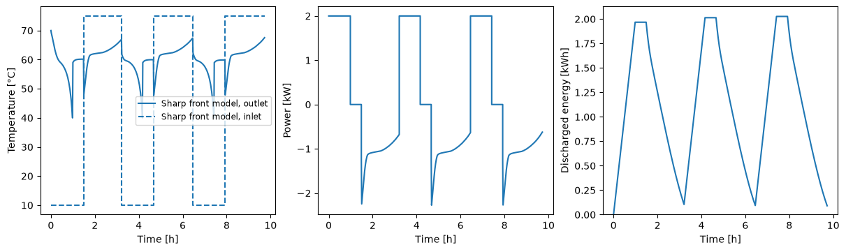
The battery starts uniform at 70 °C, and each charge ends at a slightly different state, so the discharges differ by a minute or two. During each charge the power is negative, and the discharged energy falls back as the battery takes energy in.

Time-varying conditions

A step value can also be a time series, as a 2-column array of time since the start of the step and value, interpolated linearly, or a function of that time. Here the battery supplies two draws of hot water in an hour, each of 15 minutes at 0.02 kg/s. Between the draws there is no flow, and the water left in the tube is warmed again by the PCM around it.

draws = np.array(
    [
        [0, 0.02],
        [900, 0.02],
        [901, 0],
        [1800, 0],
        [1801, 0.02],
        [2700, 0.02],
        [2701, 0],
        [3600, 0],
    ]
)
draw_solution = run_experiment(model, Experiment([s.Inlet(T_cold, draws, period=10)]))
pybamm.dynamic_plot(
    draw_solution,
    [
        ["Inlet temperature [degC]", "Outlet temperature [degC]"],
        "Mass flow rate [kg.s-1]",
        "Power [kW]",
        "Discharged energy [kWh]",
    ],
    time_unit="minutes",
);

Experiments work the same way for every model. See the experiments example for the throughputs and the round-trip efficiency over cycles, and the design study for an experiment used to compare a finned-tube battery with a packed bed.